XPS for Beginners
- XPS Course Fundamentals
- XPS Data Analysis
Welcome to the data analysis section of our XPS for Beginners course!
In part 3, we take a look at how to apply backgrounds and analysis regions to our data sets.
Open the dataset by downloading from the link above and opening in CasaXPS.
- Load the example – Ag SiO2 and fit regions to all of the elements, where appropriate
- Load the example – multi backgrounds WS2 and fit regions to all of the elements. Only fit the W 4f peaks with a background. (Check out the XPSFitting page on Tungsten to help understand the peaks)
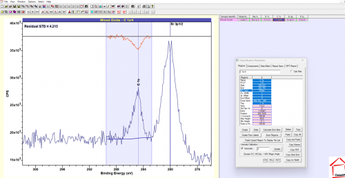
- Load the example – Mixed Oxide and apply a background to all of the elements. Put a region across ONLY the C 1s peak (Hint: Overlay the Sr 3p and C 1s spectra in Casa to help understand the peaks in this data)
Start by applying regions to the simple peaks (O 1s, Si 2p). Open quantification parameters by clicking the icon (1) or pressing F7. In the regions tab, click create to make a region (2) and then ensure the region type is ‘Shirley’. Some versions of casa, by default, will insert a Tougaard type or other background. In this case, select the ‘BG Type’ box and type ‘S’ into the box (without quotation marks) and hit enter to change to a Shirley type.
Click and drag the sides of the inserted box to move the region around the peak (1-2 eV either side).

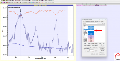
The Ag and C regions have much lower concentrations, and so the signal to noise is much poorer. In this case it may be harder to set the background through the baseline noise.
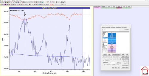
In cases such as this, we can use the ‘Average Width’ function to tell Casa to take the CPS point for the background to an average of +/- X of the selected boundary. In this case, we will set it to 3, and now our background sits in the centre of our noise much better!
Look at the N 1s peak… can we actually see anything here? No! If no peak, then we don’t need to add a region!

If we look at the W 4f spectra, we see a strange small peak near the major doublet – and by checking the details on the XPS fitting page for Tungsten we see that this is due to the W 5p emission. For this example, we will only draw a region around the W 4f peaks.
In reality, as you can see in the article above, we need to fit a background to both peaks and decouple the emissions using component fitting (to be introduced in the next lesson) – but this example is just to help you try and understand where different features may come up in close proximity and get you to apply regions to only those features you wish to analyse.

You may notice the C 1s spectra looks a little odd – so as suggested, lets overlay the Sr 3p and C 1s spectra:

If we open the Library function using the icon indicated above (or press F10) – and open the periodic table, we can find Sr and click on it to ID any Sr peaks in our data. What we can see is that we expect an Sr doublet (remember our lesson on doublets in XPS) in this region. Note that this data is uncalibrated, so the peaks are appearing at a lower energy. If we were to calibrate, we now see our peaks line up with the Sr 3p markers.

So we know that the peak at ~280 eV is actually an Sr 3p 1/2 peak!
Moving now to the C 1s block, we can apply a region to just the C 1s feature and ignore the Sr 3p contribution.
Note that this example is just for illustration, in reality there is some overlap between the two peaks and we would need to model the background as one – but this involves some advanced processes which will be covered in a later update.